How a GPS Calculates Routes

I recently bought a Garmin nüvi 40LM GPS, and I've been comparing its routes to the ones that I normally drive. There are differences, of course, some of which seem very strange until I think about the routing algorithms involved. On a whim I Googled for websites that described how those algorithms work in a consumer GPS, and didn't find anything in-depth. So here it is.

Disclaimer: I do not work for Garmin, and do not know the exact algorithms or map formats that they use. Up until this week, I did work for the company that produces the digital maps that Garmin uses. However, you won't find any trade secrets here; everything is based on publicly available documentation, well-known algorithms, and my experience implementing those algorithms.

Now that that's out of the way, the place to start is with how digital maps describe roads. Humans tend to think of roads as single continuous entities: Broad Street in Philadelphia for example. It runs 11.5 miles, from the northern border of the city to the southern border. You might think of it as North Broad and South Broad, centered on City Hall, but you wouldn't divide it further than that.

A digital map, however, divides Broad Street into hundreds of road segments, some only 30 meters long. This is because the GPS computer looks at the entire road network as a graph, with each intersection a separate node. Some maps divide the road network further: the Navteq map, for example, inserts a node wherever the speed limit changes. This makes for a lot of data; Navteq tracks over 35 million distinct road segments in North America, and more are added with each map release.

Which causes a problem for routing algorithms, because they work by walking through the graph to find the best path from start to finish. Take a look at the picture below, which is the “GridWorld” used to explain graph algorithms. There are hundreds of ways to get from point A in the upper left, to point P in the lower right.

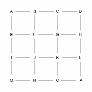
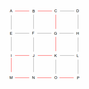
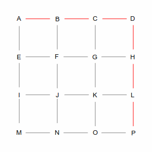
Two of those ways are shown in the following pictures. The left picture is a roundabout way, taking 10 steps, while the right picture is one of many shortest paths that take 6 steps. A simplistic algorithm would have to examine every possible route, including the roundabout ones, to discover the short ones. Not insurmountable in this example, which has only 24 streets, but in the real world of 35 million road segments, it would be impossible (or at least computationally infeasible).

Graph Traversal Algorithms

Computer scientists have been researching graph traversal algorithms for over 50 years, and have developed a variety of algorithms that do a better job than looking at every possible path. One of them, A*, is typically used for GPS routing.

The A* algorithm looks at a map much like a human would. When we want to pick a route, we mentally draw a straight line from the start to the destination, and pick roads that are close to that line. A computer can't perceive the map at a whole, but it can do something similar: when it is at an intersection (node) with multiple possibilities, it picks the node that gives the shortest total route length if it could go directly from that node to the destination. This is easier to understand with pictures.

In the first step, we have two choices: we can go from A to B or from A to E. As far as the computer is concerned they're both equivalent: there's no existing path and the direct line from each of those points to P is the same length. So it picks one arbitrarily, in this case the green path via B. But it remembers the blue path through E; you'll see why later.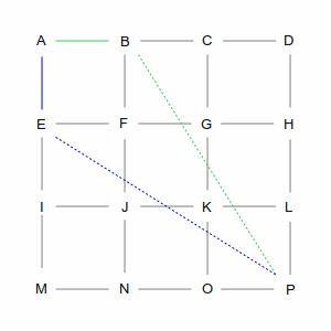
From B there are again two choices: C and F (going back to A is not an option). However, these two choices are not equivalent. The direct path from C is longer than the path from F, which makes the overall route longer, so the computer chooses F. But again, it remembers the path via C.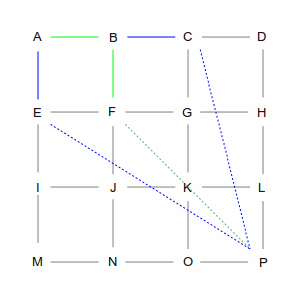
At intersection F, there are three choices: E, G, and J. But the computer remembers that it already has a path that goes through E. And since the direct line from E to P is the same no matter how you get there, it will discard — and forget — the A-B-F-E routing, because A-E is more direct. That leaves it with routes through G and J, and again, this is an arbitrary choice.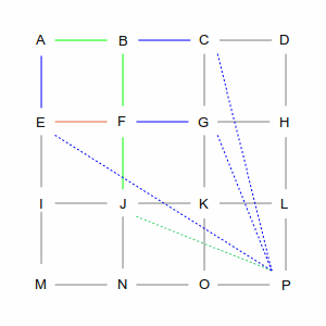
Eventually, the computer will make its way to P. Along the way it will remember several routes, and discard others, always following the shortest total path. Of course, as you've seen, this example has several shortest paths, and several places where it made an arbitrary decision. It could have just as easily picked A-B-F-G-O-P as A-B-F-J-K-L-P. What the computer would not do is pick A-B-C-D-H-L-P, even though it's the same length, because that would have taken it away from the direct line from A to P.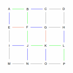

Remembered routes are also used to “backtrack” from dead ends, as in the pictures below. When the computer gets to point K, its only option is to go to G. However, it already has a path through G that is shorter. Since there's no other path, it discards the route through K and examines J and G again.

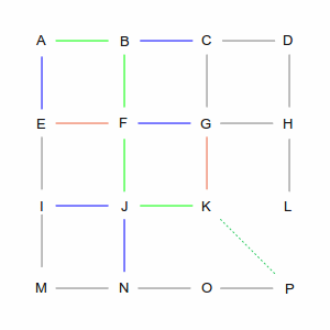
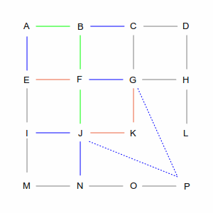
From here things get interesting, because both routes take it away from the direct line between A and P. But I think I've spent enough time in GridWorld. If you're interested, simply repeat the rule: shortest total path, combining the actual path with the calculated direct distance to the goal.

Graphs and the Real World

GridWorld is a useful way to understand graph traversal algorithms, but the real world isn't a grid — even if some people seem to wish it were. And distance is rarely the most important factor in choosing a route, elapsed time is. Given the choice between driving 50 miles on a highway and 30 on winding back roads, only motorcyclists choose the shorter route.

The simplest way to calculate elapsed time is to look at the speed limit of the road segments, and assume that traffic will move at that speed. More sophisticated implementations take into account stop signs and stoplights. If you have real-time traffic available, that becomes an important consideration as well: you don't want to get on the highway (with no way off) if you know that you'll be stopped in a five mile backup. The most sophisticated algorithms go so far as to weight right-hand turns above left-hand.

There's also the problem of CPU and memory. An exhaustive A* search works well for short routes — say five miles or less. But if you're going from Philadelphia to San Francisco, or even Philadelphia to Harrisburg, the number of remembered candidate routes would quickly use up the memory of your GPS.

To avoid this problem, digital maps classify roads based on their suitability for long-distance travel; in the Navteq map, these are known as “functional classes.” The top category (FC1) are generally interstate highways, the lowest (FC5) are neighborhood roads. In the middle are various types of highways and “arterial” roads. Of the 35 million road segments in North America, approximately 1 million are FC1 and FC2, 5 million are FC3 and FC4, and 28 million are FC5.

For long-distance routes, the GPS unit will try to find the shortest path from wherever you are to the nearest arterial. Depending on how far away your destination is, it might then follow the arterial network to the nearest limited-access highway. Once on the arterial and/or highway network, it tries to get you as close to your destination as possible. Then it steps down, from highway, to arterial, to neighborhood roads, until finding your destination. The goal is to find the destination within a hundred or so road segments; after that, the computation time and memory consumption for remembered routes becomes excessive.

Strange Choices: An Example

Once you understand how the GPS computes routes, you can explain why it doesn't do what you think it should. For example, last weekend my wife and I drove about 25 miles from our home in northwestern Philadelphia to a concert that her uncle was giving in one of the far northwestern suburbs.

On the way there, the GPS picked approximately the route that I would have: from my street (FC5) to a nearby arterial (FC4, maybe 3), to a limited-access state highway (FC2), to the PA Turnpike (FC1), exiting onto a state highway (FC3/4) and staying on it until we'd reached our destination. If I were planning the route, however, I would have skipped the arterial nearest our house and instead driven a mile to a parallel one with fewer traffic lights and less traffic. To the GPS, however, given its limited knowledge of local road conditions, the first route was better.

On the way home, the GPS did something else unexpected: it ignored the PA Turnpike, with its 65 mph speed limit, and kept us on state highways (which were generally 45 mph). Looking at a map gave a hint: the state highways almost exactly followed the line between the concert and our house. My colleague Max assures me that A* will pick the shortest route, but that's a theoretical guarantee. Inside the GPS, with its limited memory and CPU, theory has to meet practice.

There are several practical reasons for why the GPS didn't take us on the highway — and again, I don't work for Garmin, so this is pure speculation. One possibility is that it actually considered the state highway route to be shorter. In terms of absolute distance it was (24 miles versus 25), and based on the speed limits stored in the digital map, the travel time may have come out shorter as well (in practice, it took 10 minutes longer). Adding credence to this theory, there were sections of the route where the GPS displayed a 55 mph speed limit when the actual limit was 45 (incidentally, Navteq wants you to tell it where the map is wrong).

Alternatively, given the short trip distance, the GPS may have chosen to ignore the limited-access highway network. Although speed limits are higher, such highways often take you far out of the way. This means more CPU time and memory spent on finding a route from the highway to your destination, and one of the key design goals for a user interface is rapid response. That goal may trump the goal of finding the absolute shortest path. Against this theory is the fact that the GPS routed us on the highway to get to the concert.

A third possibility — and the one that I think most likely — is that the GPS will prune routes from the “open list” to minimize memory consumption. If you recall the diagrams at the start of this post, the number of “blue routes” adds up quickly. Each of these routes consumes scarce memory, so it makes sense to limit the number of paths that the GPS remembers. It's possible that one of the discarded paths is the shortest. But most people care more about getting to their destination period, rather than getting there a few minutes earlier.

Wrap-up

I'm going to finish with a bit of gushing. In my opinion, GPS is one of the most amazing examples of modern technology. A device the size of a deck of cards listens for signals from three or more satellites orbiting 12,000 miles above the earth. Then it calculate its position by comparing the different times that it took those signals (traveling at the speed of light) to arrive. Next, it figures out what road segment you're on, out of 35,000,000 possibilities, and within a fraction of a second it can tell you how to get to any other segment.

Updated December 27. Max complained that I over-simplified the explanation of A* to the point where I “should just say it's magic.” Hopefully he'll be happier with this version.

Big-O Isn't Everything

Question: when does an O(N2) algorithm outperform an O(NlogN) algorithm?

As part of my article on primitives, I decided to implement Heapsort. I needed an in-place sort for primitive integers that used an external comparator, and couldn't find one with a reasonable amount of Googling. I picked Heapsort because it's an easy algorithm to implement, and has O(NlogN) behavior for all inputs (unlike Quicksort, which degrades to O(N2) on already-sorted input unless you take care picking the pivot).

Naturally, I wanted to see how my implementation performed, vis-a-vis the sorts provided by the JDK. Particularly on large datasets, which is the reason that I wanted an in-place sort. So I created a benchmark that measured thread CPU time to sort a 10,000,000 element array (which I knew would fit in RAM). Here are the results, the average of 10 executions on my aged desktop (a 2.4 Ghz P4 with only 512 kb of cache):

Implementation	Time (sec)	Compares
Arrays.sort(int[])	2.55
Heapsort.sort(int[])	18.08
Arrays.sort(Integer[])	25.09	223,179,141
Heapsort.sort(Integer[])	79.91	439,021,125

Those are dramatic differences. I knew that Heapsort would make more comparisons than Mergesort (which the JDK will use for Integer[]), so I added a counter to the comparator. But the running time was over three times longer, with only twice the number of comparisons. And Quicksort (used by the JDK for int[]) was over seven times faster. Perhaps some of that difference comes from Heapsort calling a comparator, but clearly, not all O(NlogN) algorithms are alike!

So I decided to look at the JDK source. And found this interesting bit of code:*

private static void sort1(int x[], int off, int len) {
// Insertion sort on smallest arrays
if (len < 7) {
    for (int i=off; i<len+off; i++)
    for (int j=i; j>off && x[j-1]>x[j]; j--)
        swap(x, j, j-1);
    return;
}

Insertion sort is an O(N2) algorithm. But it doesn't have a lot of moving parts — unlike Quicksort, which takes almost 40 lines of code in the JDK implementation, not counting the swap and range-swap methods. And when N is small, lines of code are more important than algorithmic efficiency (or, as my coworker Max points out, when N is bounded, you have a constant-time operation).

There's one more performance-enhancing feature of this snippet: all of the data accesses should be within the L1 cache. On Intel processors, the cache is structured as 64-byte chunks of memory — enough to hold 8 adjacent int values. While Arrays.sort() makes no attempt to ensure alignment of the insertion-sorted sub-arrays, it's a naturally cache-friendly algorithm. As is Quicksort itself, for that matter. And Heapsort, which jumps around the array comparing elements at position N and 2 * N, is decidedly cache-unfriendly.

All of which is to say that sometimes, micro-optimizations have a big effect. And that, rather than implementing Heapsort, I should have simply copied the OpenJDK implementation of Quicksort and added a comparator.**

---

* This optimization isn't specific to the JDK. The GNU C library implementation also switches to insertion sort, albeit at 4 elements, and credits Sedgewick for that and other optimizations.

** In case you're wondering, the updated Quicksort took 4.25 seconds to run, and made approximately 375,000,000 comparisons. If it weren't covered by GPL2, I'd put it in my toolbox in place of the Heapsort implementation.